5 Charts To Watch

Introduction

Our high-level investment view for this year is that a combination of improving global growth boosting profits and still easy monetary conditions will help drive reasonable investment returns, albeit more modest than the very strong gains of 2019. This note revisits five charts we see as critical to the outlook.

Chart #1 Global business conditions PMIs

Global Purchasing Managers Indexes (PMIs) – surveys of purchasing managers at businesses in most major countries – are an excellent and timely guide to the state of the global economy. Although services sector PMIs held up better than for manufacturers – which tend to be more cyclical – both softened through 2018 and into mid-2019. Since then they have shown signs of improvement suggesting that the global monetary easing seen through 2019 with interest rate cuts and renewed quantitative easing is working. Going forward they will need to improve further to be consistent with our view that growth will pick up this year.

But so far, the 2018-19 slowdown in business conditions PMIs (and hence global growth) looks like the slowdowns around 2012 and 2015-16 as opposed to the recession associated with the global financial crisis (GFC).

Chart 2 Global inflation

Major economic downturns are invariably preceded by a rise in inflation to above central bank targets causing central banks to slam the brakes on. At present, core inflation – ie inflation excluding the volatile items of food and energy – in major global economies remains benign. In the US, the Eurozone and Japan core inflation is well below their central bank targets of 2%. Inflation in China spiked to 4.5% through last year, but core inflation has been falling to 1.4% and is well below the Government’s 3% target/forecast. A clear upswing in core inflation would be a warning sign that spare capacity has been used up, that monetary easing has gone too far, and that the next move will be aggressive monetary tightening. But at present we are a long way from that.

Chart 3 – The US yield curve

The yield curve is a guide to the stance of monetary policy. When short-term interest rates are low relative to long-term rates businesses can borrow short and lend (or invest) long and this grows the economy. But it’s not so good when short rates are above long rates. An inverted US yield curve has preceded past US recessions. So, when this happened last year there was much concern that a US recession was on the way. However, in recent months various versions of the yield curve – with the gap between the US 10 year bond yield and the Fed Funds rate and the US 10 year bond yield and the 2 year bond yield shown in the next chart – have uninverted as the Fed cut rates and hence short-term yields fell, good economic data provided confidence that recession will be avoided and the US/China trade war de-escalated reducing the threat posed by the trade war.

While the US yield curve has uninverted in the past and yet a recession has still come along, the uninversion seen in recent months coming after such a shallow and short-lived inversion provides confidence that the inversion seen last year gave a false signal as occurred in the mid to late 1990s (as circled).  In addition, it’s also worth noting that other indicators suggest that US monetary policy was far from tight – the real Fed Fund rate was barely positive, and the nominal Fed Funds rate was well below nominal GDP growth and both are far from levels that in the past have preceded US recessions.  So it’s a good sign that the US yield curve has been steepening in recent months. A return to yield curve inversion – which became deeper than seen last year – would be a concern of course.

Chart 4 – The US dollar

Moves in the value of the US dollar against a range of currencies are of broad global significance. This is for two reasons. First, because of the relatively low exposure of the US economy to cyclical sectors like manufacturing and materials the $US tends to be a “risk-off” currency, ie it goes up when there are worries about global growth. Second, because of its reserve currency status and that a lot of global debt is denominated in US dollars particularly in emerging countries, when the $US goes up it makes it tough for emerging countries.

So when global uncertainty is rising this pushes the $US up which in turn makes it hard for emerging countries with $US denominated debt. If we are right though and global growth picks up a bit, trade war risk remains in abeyance and the Iran conflict does not become big enough to derail things then the $US is likely to decline further which would be positive for emerging countries.

Chart 5 – World trade growth

It’s reasonable to expect growth in world trade to slow over time as services become an ever-greater share of economic activity and manufacturing becomes less labour dependent. However, President Trump’s trade wars since 2018 combined with slower global growth saw global trade fall last year. This year should see some reversal if the trade wars remain in abeyance as Trump focuses on keeping the US economy strong to aid his re-election and global growth picks up a bit.

US recession still a way away

In recent years there has been much debate about whether a new major bear market in shares is approaching. Such concerns usually reach fever pitch after share markets have already fallen 20% or so (as they did into 2011, 2016 and 2018). The historical experience tells us that what happens in the US is critical to how deep share market falls get. Deep (“grizzly”) bear markets like the 50% plus fall seen in the GFC are invariably associated with US recession. So, whether a recession is imminent in the US, and more broadly globally, is critically important in terms of whether a major bear market is on the way. The next table summarises the key indicators we are still watching in this regard.

US recession signposts

Indicator Recession Yes/No
Yield curve inverted ?
Fed Funds rate well above growth No
Cyclical spending, % of GDP No
Private debt growth No
US leading indicator No
Inflation well above target No

Source: AMP Capital

These indicators are still not foreshadowing an imminent recession in the US. The yield curve is most at risk if it inverts again. But other measures of monetary policy in the US are not tight and we have not seen the sort of excesses that normally precede recessions – discretionary or cyclical spending as a share of GDP is low, private debt growth has not been excessive, the US leading indicator is far from recessionary levels and inflation is benign.

Concluding comments

At present, most of these charts or indicators are moving in the right direction, with the PMIs improving a bit, inflation remaining low, the yield curve steepening, the $US showing signs of topping and the US/China trade truce auguring well for some pick up in world trade growth. But to be consistent with our view that this year will see good returns from shares we need to see further improvement and so these charts are worth keeping an eye on.

Dr Shane Oliver

Head of Investment Strategy and Chief Economist

AMP Capital

Review of 2019, Outlook for 2020

2019 – Growth Down, Returns Up

Christmas 2018 was not a great one for many investors with an almost 20% slump in US shares from their high in September to their low on Christmas Eve, capping off a year of bad returns from share markets and leading to much trepidation as to what 2019 would hold. But 2019 has turned out to be a good year for investors, defying the gloom of a year ago. In fact, some might see it as perverse – given all the bad news around and the hand wringing about recession, high debt levels, inequality and the rise of populist leaders. Then again that’s often the way markets work – bottoming when everyone is gloomy then climbing a wall of worry. The big global negatives of 2019 were:

  • The trade war and escalating US-China tensions generally. A trade truce and talks collapsed several times leading to a new ratcheting up of tariffs before new talks into year end.
  • Middle East tensions flared periodically but without a lasting global impact & the Brexit saga dragged on although a near-term hard Brexit looks to have been avoided.
  • Slowing growth in China to 6%. This largely reflected an earlier credit tightening, but the trade war also impacted.
  • Slowing global growth as the trade war depressed investment & combined with an inventory downturn and tougher auto emissions to weigh on manufacturing & profits.
  • Recession obsession with “inverted yield curves” – many saw the growth slowdown as turning into a recession.

But it wasn’t all negative as the growth slowdown & low inflation saw central banks ease, with the Fed cutting three times and the ECB reinstating quantitative easing. This was the big difference with 2018 which saw monetary tightening.

Australia also saw growth slow – to below 2% – as the housing construction downturn, weak consumer spending and investment and the drought all weighed. This in turn saw unemployment and underemployment drift up, wages growth remain weak and inflation remain below target. As a result, the RBA was forced to change course and cut interest rates three times from June and to contemplate quantitative easing. The two big surprises in Australia were the re-election of the Coalition Government which provided policy continuity and the rebound in the housing market from mid-year. While much of the news was bad, monetary easing and the prospect it provided for stronger growth ahead combined with the low starting point resulted in strong returns for investors. 

  • Global shares saw strong gains as markets recovered from their 2018 slump, bond yields fell making shares very cheap and monetary conditions eased. This was despite several trade related setbacks along the way. Global share returns were boosted on an unhedged basis because the $A fell.
  • Emerging market shares did well but lagged given their greater exposure to trade and manufacturing and a still rising $US along with political problems in some countries.
  • Australian share prices finally surpassed their 2007 record high thanks to the strong global lead, monetary easing and support for yield sensitive sectors from low bond yields.
  • Government bonds had strong returns as bond yields fell as inflation and growth slowed, central banks cut rates and quantitative easing returned. • Real estate investment trusts were strong on the back of lower bonds yields and monetary easing.
  • Unlisted commercial property and infrastructure continued to do well as investors sought their still relatively high yields. However, Australian retail property suffered a correction.
  • Commodity prices rose with oil & iron up but metals down.
  • Australian house prices fell further into mid-year before rebounding as the Federal election removed the threat to negative gearing & the capital gains tax discount, the RBA cut interest rates and the 7% mortgage test was relaxed.
  • Cash and bank term deposit returns were poor reflecting new record low RBA interest rates.
  • The $A fell with a lower interest rates and a strong $US.
  • Reflecting strong gains in most assets, balanced superannuation funds look to have seen strong returns.

2020 Vision – Growth Up, returns still good

The global slowdown still looks like the mini slowdowns around 2012 and 2015-16. Business conditions indicators have slowed but remain far from GFC levels. See next chart.

While the slowdown has persisted for longer than we expected – mostly due to President Trump’s escalating trade wars – a global recession remains unlikely, barring a major external shock. The normal excesses that precede recessions like high inflation, rapid growth in debt or excessive investment have not been present in the US and globally. While global monetary conditions tightened in 2018, they remained far from tight and the associated “inversion” in yield curves has been very shallow and brief. And monetary conditions have now turned very easy again with a significant proportion of central banks easing this year. See chart. The big global themes for 2020 are likely to be:

  • A pause in the trade war but geopolitical risk to remain high. The risks remain high on the trade front – with President Trump still ramping up mini tariffs on various countries to sound tough to his base and uncertainty about a deal with China, but he is likely to tone it down through much of 2020 to reduce the risk to the US economy knowing that if he lets it slide into recession and/or unemployment rise he likely won’t get re-elected. A “hard Brexit” is also unlikely albeit risks remain. That said geopolitical risks will remain high given the rise of populism and continuing tensions between the US & China. In particular, the US election will be an increasing focus if a hard-left candidate wins the Democrat nomination.
  • Global growth to stabilise and turn up. Global business conditions PMIs have actually increased over the last few months suggesting that monetary easing may be getting traction. Global growth is likely to average around 3.3% in 2020, up from around 3% in 2019. Overall, this should support reasonable global profit growth.
  • Continuing low inflation and low interest rates. While global growth is likely to pick up it won’t be overly strong and so spare capacity will remain. Which means that inflationary pressure will remain low. In turn this points to continuing easy monetary conditions globally, with some risk that the Fed may have a fourth rate cut.
  • The US dollar is expected to peak and head down. During times of uncertainty and slowing global growth like over the last two years the $US tends to strengthen partly reflecting the lower exposure of the US economy to cyclical sectors like manufacturing and materials. This is likely to reverse in the year ahead as cyclical sectors improve.

In Australia, strength in infrastructure spending and exports will help keep the economy growing but it’s likely to remain constrained to around 2% by the housing construction downturn, subdued consumer spending and the drought. This is likely to see unemployment drift up, wages growth remain weak and underlying inflation remain below 2%. With the economy remaining well below full employment and the inflation target, the RBA is expected to cut the official cash rate to 0.25% by March, & undertake quantitative easing by mid-year, unless the May budget sees significant fiscal stimulus. Some uptick in growth is likely later in the year as housing construction bottoms, stimulus impacts and stronger global growth helps.

Implications for Investors

Improved global growth and still easy monetary conditions should drive reasonable investment returns through 2020 but they are likely to be more modest than the double-digit gains of 2019 as the starting point of higher valuations and geopolitical risks are likely to constrain gains & create some volatility: •

  • Global shares are expected to see returns around 9.5% helped by better growth and easy monetary policy.
  • Cyclical, non-US and emerging market shares are likely to outperform, particularly if the US dollar declines and trade threat recedes as we expect.
  • Australian shares are likely to do okay but with returns also constrained to around 9% given sub-par economic & profit growth. Expect the ASX 200 to reach 7000 by end 2019.
  • Low starting point yields and a slight rise in yields through the year are likely to result in low returns from bonds.
  • Unlisted commercial property and infrastructure are likely to continue benefitting from the search for yield but the decline in retail property values will still weigh on property returns.
  • National capital city house prices are expected to see continued strong gains into early 2020 on the back of pent up demand, rate cuts and the fear of missing out. However, poor affordability, the weak economy and still tight lending standards are expected to see the pace of gains slow leaving property prices up 10% for the year as a whole.
  • Cash & bank deposits are likely to provide very poor returns.
  • The $A is likely to fall to around $US0.65 as the RBA eases further but then drift up a bit as global growth improves to end 2019 little changed.

What to Watch?

The main things to keep an eye on in 2020 are as follows:

  • The US trade wars – we are assuming some sort of de- escalation in the run up to the presidential election, but Trump is Trump and often can’t help but throw grenades.
  • US politics: the Senate is unlikely to remove Trump from office if the House votes to impeach and another shutdown is also unlikely but both could cause volatility as could the US election if a hard-left Democrat gets up (albeit unlikely).
  • A hard Brexit looks like being avoided but watch UK/EU free trade negotiations through the year.
  • Global growth indicators – like the PMI shown in the chart above need to keep rising.
  • Chinese growth – a continued slowing in China would be a major concern for global growth.
  • Monetary v fiscal stimulus in Australia – significant fiscal stimulus could head off further RBA rate cuts and quantitative easing.

Written by Dr Shane Oliver Chief Economist at AMP Capital

Where is the Value?

Investing can be seen as difficult and there are many schools of thought as to the best approach.  The APC Investment Philosophy taps into academic research which incorporates a number of guiding principles, such as investing is not speculating.  Another of which is the relationship between risk and return, which results in a methodical and disciplined ‘tilting’ of share investments towards ‘small cap stocks’ as well as ‘value stocks’.

At the APC Annual Client Briefing held in August (link here) we took a closer look at the performance of these ‘tilts’ with a key finding that the ‘value premium’ sought had deserted us in recent history, impacting short term returns.  Taking a deeper dive, this is however not an uncommon occurrence when we look at a longer period.  History has shown us that ‘value’ stocks underperformed the broader market 13% of the time in Australian markets and 17% in international markets in the 10 years up until December 2018. 

If we were to look further back, ‘value’ stocks had underperformed ‘growth’ stocks by an average of nearly 6% per year for the 10 years ending 31 March 2000 leading to some at the time questioning whether the ‘value premium’ was a reliable source of excess returns and if it would be possible to recover this lost ground.  Fast forward to the beginning of March 2001 (only 12 months later) and the recovery of ‘value’ stocks was such that the 10 year number had reverted from a negative to a positive with ‘value’ outperforming ‘growth’ by nearly 40% from April 2000 to February 2001.

While the value premium will seemingly ‘disappear’ from time to time it’s important to keep a long term view.  While the above demonstrates the extremes, the tilt to ‘value’ stocks in portfolios has in the fullness of time, historically, resulted in an average outperformance as evidenced in our presentation. 

As it happened, there has been a recent swing in the fortunes of ‘value’ stocks with the three months following the APC Annual Client Briefing showing ‘value’ stocks outperforming ‘growth’ stocks by over 2% globally.

Not for one instance are we suggesting a recurrence of the numbers leading up to February 2001 is on the cards but maybe Santa is a ‘value’ investor.  Investment markets can move quickly and trying to chase the best returns can often lead to investment misery – sticking to the plan and long term fundamentals is by far the better strategy.

The Espresso Portfolio

Written By Jim Parker for “Outside the Flags”.

When you haven’t got much capital of your own, the road to financial security can seem long, hard and complex. But the truth is that wealth building is relatively simple. All it takes is time and the price of a cup of coffee.

A son of a friend just graduated from university. Still in his early 20s and with student loans to pay off, Josh has hardly any savings or capacity to save much at all. So Josh and I met for coffee and a chat. He had acquired a taste for espresso while studying and working at night waiting tables. (The coffee kept him awake).

“How much do you spend on espresso each week?” I asked him. After thinking for a moment, he replied that he averaged about two cups a day, each costing $3. That equated to about $40 a week or $160 a month. “Well, what if you sacrificed the coffee and put the cash into a savings scheme instead?” I suggested.

Josh looked doubtful. Kicking caffeine wouldn’t be easy. Besides, he couldn’t imagine that loose change spent on coffee would make much difference to his long-term financial position. I dealt with the first problem by suggesting he make instant coffee at home and bring it into work each day in a flask. The second problem – that it wouldn’t be effective – I dealt with by telling him about the miracle of compounding.

With initial balance of $100, a monthly contribution of $160 and a yield of 5%, his coffee money would gradually accumulate to a pool of a quarter of a million dollars by the time of his retirement. And this was without saving another cent.
Assuming Josh’s salary was to rise on his graduation, he might bump up that monthly contribution to $500.

In this case, his savings pool would grow to three quarters of a million by his retirement. And this was a conservative estimate.

This sounds too easy, he said. That’s because it is easy, I replied. The interest he earned on his saving was paid into his account and included in the next calculation. So he was earning interest on interest. The key was that firstly he was starting early. Secondly, he was saving a small amount consistently month after month. Thirdly, he was exercising patience. The rest of it was just the effect of time and compounding. (Obviously, this young man’s earnings will be subject to tax. But the purpose of this exercise was to show him that a small sacrifice, made regularly, would yield significant results over time.)

Josh now refers to his savings plan as his ‘espresso portfolio’. The initial pain of kicking his expensive caffeine habit was made up for by the slow roast of a savings scheme that promised him a comfortable retirement.

Even for those of us much older than Josh, there are lessons here. We tend to underestimate the effect of gradual saving and patience in building wealth, just as we tend to over-rate gimmicks promoted in the media. We can’t control the ups and downs of markets or the daily noise of the media. We can control our own behaviour.

Now enough of this talk about money. How about a coffee? It’s on me.

The nuts and bolts of the First Home Loan Deposit Scheme

Housing affordability continues to sit atop the list of hard-to-solve political issues in Australia. In late October, the government gave the first insight into the mechanics of the First Home Loan Deposit Scheme (FHLDS), its latest attempt to ease the struggle many young Australians face when looking to buy their first home.

Last month, Treasury released an exposure draft of the investment mandate that would govern the FHLDS. This draft mandate was finalised on November 11, 2019 without significant amendment. With this in mind, we will first look at the nuts and bolts of the FHLDS in November’s Technical Journal. In this month’s Industry Insights we focus on the historical context of the FHLDS, as well as some of the potential issues with, and opportunities presented by, the scheme.

So, let’s start with how the scheme will work.

The scheme in a nutshell

Under the scheme, the National Housing Finance and Investment Corporation (NHFIC) will provide a guarantee to help eligible first home buyers increase their security amount on the purchase of their first home to 20 per cent. First home buyers need to meet an income test, the purchased home needs to be valued below set thresholds and the first home buyer(s) need to have at least 5 per cent of the home’s value as a deposit.

The scheme will commence on January 1, 2020 and a limit of 10,000 guarantees per financial year applies. Guarantees would be applied on a first-come, first-served basis.

In practice
The NHFIC provides a guarantee that increases the borrower’s security to 20 per cent of the value of the property at purchase. So, if the borrower has a 5 per cent deposit, the guarantee is for a further 15 per cent. If the borrower has 10 per cent, the guarantee is for 10 per cent and so on. By lifting the borrower’s security amount to 20%, the lender should no longer require the borrower to take out mortgage protection insurance. The cost of such insurance can vary from hundreds to thousands of dollars a year, depending on the age of the life insured, the size of the loan and associated repayments, and the events covered.

For a loan to be eligible for the scheme, it needs to meet the following criteria:

  1. It is provided by an eligible lender,
  2. There are no more than two borrowers,
  3. If there are two borrowers, they are spouses or de facto partners,
  4. Each owner is a first home buyer and will occupy the home,
  5. The loan is to purchase residential property which does not exceed the price cap,
  6. Loan repayments are on a principal and interest basis and the term does not exceed 30 years (although an interest-only period is permissible where the loan relates to the building of a new residence),
  7. If the loan is to buy land it must also be to build a home on the land,
  8. The loan to value ratio is between 80 and 95 per cent.

In practice
For an FHLDS guarantee to apply to a loan issued to the maximum of two borrowers, the borrowers must be in a spousal, or de facto, relationship. This is in contrast to the conditions of the First Home Super Saver scheme, where more than 2 joint purchasers can pool their funds and no specific relationship between the purchasers is required.

Eligible Loans

If a loan is already approved for the scheme, it can be refinanced, and the scheme will continue to apply to it.

There are limits on how many FHLDS guarantees can be applied to loans issued by the big four banks (Westpac, NAB, ANZ and Commonwealth Bank). Only two of these banks may have any FHLDS guarantees applied to their loans in a given financial year, and a maximum 5,000 guarantees may be applied to loans from those two banks.

First home buyer

In order to qualify for the scheme, each owner of the home purchased with the loan must:

The income test

The income test is applied to the financial year preceding the year the loan agreement is entered into and assesses taxable income. To qualify for the scheme, such income cannot exceed:

  • $200,000 combined for couples, or
  • $125,000 for singles.

Price cap

FHLDS guarantees can only be applied to loans on properties that do not exceed the price cap for that region.

The price cap for the calendar year is determined by the NHFIC each January 1. The investment mandate applies the price cap at commencement as:

  • ACT – $500,000
  • Sydney, Illawarra, Newcastle and Lake Macquarie – $700,000
  • Other NSW – $450,000
  • Melbourne and Geelong – $600,000
  • Other Vic – $375,000
  • Brisbane, Sunshine Coast and Gold Coast – $475,000
  • Other Qld – $400,000
  • NT – $375,000
  • Adelaide – $400,000
  • Other SA – $250,000
  • Perth – $400,000
  • Other WA – $300,000
  • Hobart – $400,000
  • Other Tas – $300,000
  • Jervis Bay and Norfolk Island – $450,000
  • Christmas Island and Cocos (Keeling) Islands – $300,000

The definition of cities and regional centres listed is taken from the Australian Statistical Geography Standard. Regional centres are defined as those in Statistical Area Level 4. An interactive map provided by the ABS is available here.

Value

The value of a property is taken at the time the loan contract is entered into, and is the value of the property assessed by the lender. This may be different to the market value at which the property was purchased.

Guarantee limit

The NHFIC’s guarantee under the scheme is limited to 20 per cent of the value of the property, less the deposit paid by the purchaser(s). The guarantee ceases when the outstanding loan amount is less than 80 per cent of the value of the property as assessed by the lender at the time of purchase.

The scheme will not be a financial product

Along with the draft mandate, draft regulations were consulted upon by Treasury that would exempt the scheme from being considered a financial product. As such, the recommendation that a client apply for a FHLDS guarantee will be free from the compliance requirements attached to advice on a financial product.

Under the National Consumer Credit Protection Act 2009, the FHLDS does not seem to represent credit either. As the borrower has no obligation to repay the government for their guarantee, no debt  to the government is incurred or deferred. That said, the loan to which the FHLDS guarantee is applied is most certainly credit, and for an adviser to provide any specific guidance on the loan to a client, they will need to operate under an Australian Credit Licence.

Change is inevitable

The investment mandate may well be subject to change before the FHLDS is launched. That said, the current rules do provide a good insight into the broader shape of the scheme and how it will apply to clients. Keep an eye out for this month’s Industry Insights where will discuss some of the deeper issues arising from the FHLDS.

Has Anyone Seen the Value Premium?

Extending on Hayden’s discussion regarding the Value premium at our Annual Client Briefing here is another independent article found on this issue that APC feels might be of interest to some of our clients.

Written and researched by GARRETT QUIGLEY and posted on the evidence based investor website September 2019;

There has been plenty of commentary recently on the fact that value has been underperforming growth. We wrote a piece on this in 2016 when we showed that standard value/growth indices were then indicating that value had underperformed growth over the prior 10-year period by 1.1% p.a. Here we update this data and introduce some related topics which we will consider over the coming months.

For our returns and characteristics data, we use a well-known source of independent data provided by Style Analytics. Using their analysis tools, we create portfolios based on book-to-market (B/M), which is a standard metric for sorting stocks on value-versus-growth, and then track the returns and characteristics of these simulated portfolios through time. For our purposes here, we create global portfolios where we capture the top 30% (Value) and the bottom 30% (Growth) by market value of stocks when ranked by B/M. We set the country weights in each portfolio to match their market weights in a broad index. We also exclude the bottom 5% of each market to avoid any potential distortions due to micro-cap stocks. All returns are in UK sterling,

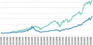
We start the portfolios at the end of 1989 (if we go further back than this, the data coverage declines). A chart of the returns is shown in the figure below,

Total Return of Value and Growth Portfolios since January 1990 (in GBP)


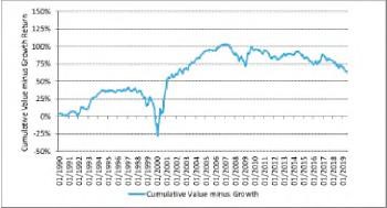
To track the relative returns of Value versus Growth, each month we subtract the return of the global Growth portfolio from the global Value portfolio, and we cumulate that sum through time as shown in the chart below. As the chart shows, the relative return of Value versus Growth has been declining recently – i.e. value stocks have been doing relatively worse than growth stocks globally, and this continues a trend that has been apparent for some years. Indeed, the negative trend has continued since we wrote about it in 2016.

The Ft*lath’s Performance of Value vs. Growth Stock Portfolios


This has caused some commentators to worry about Value as a factor in general and others to argue that now is a good time to rotate portfolios towards Value. However, a key issue that is worth considering here is the degree to which the respective ratings of Value and Growth stocks have changed over time. One proxy for this is the Price-to-Book ratio of each portfolio. Price-to-Book or P/B is simply the inverse of B/M but is somewhat more intuitive and is generally preferred as a metric by investors.

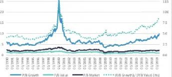
The chart below shows the P/B ratio of the Growth and Value portfolios constructed as above as well as that of the overall market, all as solid lines using the left-hand scale. It is clear from this chart that the P/B ratio of Growth stocks has been trending up since the onset of Quantitative Easing (OE) in early 2009 and is now at 9.8 on a weighted average basis versus a long run average of 6.67 over the nearly 30-year period covered below. Growth stocks are now trading at a rating similar to that prevailing in late 1999 in the middle of the Tech boom. Of course, Tech stocks are much more profitable now compared to then, but on a P/B basis, they are trading at a historically high level.

Since the onset of QE, Value stocks have not been bid up anything like as much as Growth stocks. In fact, they trade at a P/B of 1.12 compared to their long run average P/B of 1.27, hence at a small discount to that long run average. This change in the rating spread between Growth and Value stocks is shown in the dotted line on the chart below (and maps to the scale on the right-hand side). This dotted line is simply the ratio of the P/B of Growth stocks divided by that of Value stocks. As of the end of July this year, the P/B spread is 8.74 and as the chart shows, it is at a level that looks extremely stretched historically.

Price-to-Book Ratios of Global Value and Growth Portfolios


Some of these ratios are shown over the last 10 and 20 years in the table below. In Panel 1, the P/B ratios are shown for Growth and Value stocks, and the Spread (here shown as the ratio of the P/B of Growth divided by the P/B of Value) is shown on the rightmost column. The changes in P/B are shown in Panel 2. For example, over the last 10-year period, the P/B of Growth stocks increased by 131% whereas the P/B of Value stocks increased by only 23%. The annualised change in the P/B ratios is shown on the right of Panel 2. So over 10-years, the Growth stock portfolio experienced an annualised uplift in its P/B ratio of 8.7% p.a. compared to just 2.1% for Value stocks.

From Panel 3, we can infer the effect of the P/B changes on returns. Over the last 10 years, Growth stocks had a total return of 325%, equivalent to 15.6% p.a. and Value stocks returned 213%, or 12.1% p.a, a difference of 3.5% p.a. in favour of Growth stocks. However, as we saw in Panel 2, Growth stocks have also been substantially rerated – at least insofar as their P/B ratios have been pushed higher indicating high future return expectations.

On the right of Panel 3, we show the effect of deducting the rating change from the return of Growth and Value portfolios over 10- and 20-year periods. For example, the 15.6% return for Growth stocks over the last 10 years is reduced to 6.8% after adjusting for the 8.7% p.a. rating change etc. Value stocks on the other hand had a smaller uplift in their P/B level of just 2.1% p.a. so when this deducted from the 10-year Value return the adjusted return is 10%, which is 3.2% higher than the adjusted Growth return.


Of course, this is a rather crude rating adjustment and there are other metrics that one might consider as well as the current and expected levels of profitability of Growth versus Value stocks. The broader point is that Growth stocks may have done relatively well over a sustained period, and this has occurred once before in the last 30-year period. However, the last time Growth stocks traded at this high a level was in late 1999. We can see from the top chart and Panel 3 of the table that over the 20-year period since mid-1999, when the P/B spread was at 6.4, less than it is now, Growth stocks underperformed value stocks by 2.1% p.a. This was in spite of the fact that over the 20-year period, Value stocks were pulled down by a greater decrease in their P/13 level.

It is unwise to think that markets will repeat these patterns in a simple way, especially since we are in unusual times with $15 trillion of government and corporate debt across the world exhibiting negative yields. However, it is equally unwise to be influenced too much by recent relative performance. Doing so would have led to very poor asset allocations historically and the simple fact remains that valuation still serves as a useful, if imperfect, guide to long-run expected returns

APC’s LaTrobe University Scholarship

As you will know Australian Private Capital has provided a scholarship at La Trobe University for a number of years.  In order to be considered, the recipient needs to live outside of Melbourne and be intending to study in a finance related field. 

The reason why APC provides this financial support is we recognise that relocating to Melbourne to study is a difficult endeavour for many.  Being away from family and friends is not easy and the financial burden can place a strain undermining the student’s focus on their studies.

This year, our scholarship is being awarded to Luh Emi Purnama Madrini.  Luh became interested in business and finance when he completed VCE studies in Business and Accounting which lead him to enrol in La Trobe’s VCE Plus program.

Luh commenced a Bachelor of Commerce at La Trobe and has since transferred to a double Commerce / Law degree.  Luh’s decision to study at La Trobe has a historical family link as his father studied at La Trobe.  Growing up as a farmer in an extremely disadvantaged village in Indonesia, Luh’s father himself received scholarships to study at La Trobe and provided him the means and opportunity to break the cycle of poverty.

The impact of these scholarships has had enormous benefits for Luh’s father and his family, allowing other family members to come to Australia and study.

This experience illustrates the power of education and business opportunity to break the cycle of poverty.  This notion of ‘Business being a force for immense good in the world’ has motivated APC over many years in our supportive endeavours at both Melbourne Business School and La Trobe University and is something we are very proud to continue to do.